Field Activity #2: Conducting a Distance Azimuth Survey

Introduction:

The second exercise of the course dealt with the surveying of a grid based coordinate system on small plots. In order to have a quality survey, a geographer needs to have precise GPS technology. However, in some cases this technology can not always be relied on, and therefore one needs to improvise. By using various hand-held tools to measure distances and azimuths one ran coordinate different points to create a map. In this case the latitude and longitude will only be given for the base points of which one stands. The surrounding trees will all be mapped according to the distance from that origin point.

Study Area:

This Field Activity was done on Putnam trail, which is located south of Phillips hall (see figure 1). The base points were roughly 300-400 feet from the back of Phillips. Data was collected from standing on the dirt path, and picking ten of the surrounding trees for the measurements. The trees utilized for data collection were chosen by the groups rotating 360 degrees without moving from the base point. The red path below is rough estimate of the Putnam trail location.

Figure 1 displays the study area of the Distance Azimuth Survey.

Methods:

In order to get the survey results, each group had to record the latitude and longitude of the base point, the azimuth of the tree from the origin spot, the circumference of the tree, and the distance from the base point. The gadgets this class used to help obtain these statistics were: a GPS, a hand-held laser measure, a measuring tap, and a azimuth compass. This group also recorded the tree types thanks to the professor's guidance.

Figure 2 displays the hand-held
 azimuth compass

The instrument we used to measure the azimuth is shown in Figure 2. By looking through through a hole in the bottom, and keeping both eyes open, one can see the degree of each trees location relevant to the origin spot.

Figure 3 shows the GPS used to
mark the two origin locations

The GPS unit, shown in Figure 3 was used to record the location for both origin points in the survey. Due to the low-technology of the given GPS make sure to write down the coordinates in a hard copy.

Figure 4 displays the Measuring Tape

The measuring tape in Figure 4 was used to measure the circumference of the tree in meters. This is one the of the quickest and simplest ways to record the circumference.

Figure 5 Displays the hand-held laser
measuring device

 The last gadget used during the survey was the hand-held laser   measuring device, shown in Figure 5. Aiming the laser pointer   directly at a tree will show the exact distance from the the origin   spot to that tree in meters.




Each group used the previously explained techniques to collect the data on ten different trees at two different base points. Once all data for the Distance azimuth survey is recorded, it needs to be entered into a Microsoft office excel sheet, and then imported to Arc Map (shown in Table 1).

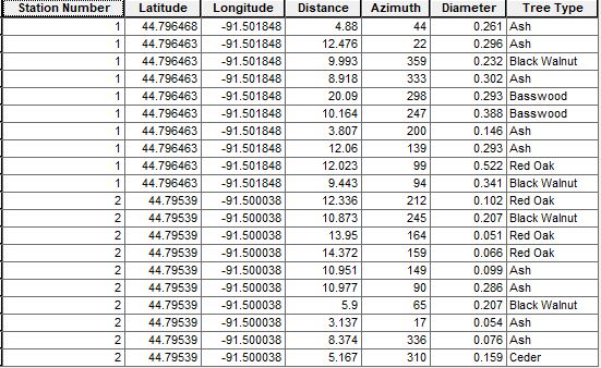Table 1 displays the full results of the data recorded from the two base points

Importing the Data into ArcMap:

Figure 6 displays the data inputted into the correct field

Bring the table into the layers column under table of contents. Right click the table and choose display X and Y coordinates to make sure everything will match up. To help verify the accuracy even more bring in a base map. If the coordinates all match you, then click on the Bearing Distance to Line command out of the arc toolbox under Data Management tools in the Features category to import the rest of the data (see Figure 6). This tool creates a new feature class using the latitude and longitude coordinate fields values giving you geodetic line features. Once the correct information is entered click "OK". Then ten poly lines will appear branching off each base point to the approximate tree location.


After that utilize the Feature Vertices to Points command also in the arc toolbox. This tool can be found ten or so tools down from the Bearing Distance to Line command tool, but you can also just search for it. This tool will allow you to create a new feature class made up of points that are generated from specific locations. Enter the new tree feature class under input features, choose a name under output feature class, and lastly select end for the point type. The points will be placed on the end of the polylines created by the Bearing Distance to Line command. Then right click on the newly created feature class, go to properties, and under 'symbol' make a proportional symbol map based off the tree diameter. Any maps created must include a north arrow, a scale bar, a locator map, a watermark, and a data source.

Results: 

Once you have completed all the steps under the methods subheading, the results will be ready. This group had very few complications while completing the methodology portion, but going through the previously explained methods above, the solution to any issues should be obtainable. As you can see in Figure 7, this distance azimuth survey proved that by using a compass, a laser pointer, a measuring tape, and a azimuth recorder, a fairly accurate map can be produced. Any inaccurate data can be blamed on human error, but for the most part all the trees seem to be the exact distance away from the base point as they were in the field.

Figure 7 displays the final map created emphasizing on Tree Diameter.

Figure 8 shows a county level view of the study area

Conclusion:

After completing the Distance Azimuth survey, the grid based coordinate system proved to be an accurate way to map the necessary technology isn't working. It is a simple technique, making it easy to acquire the data necessary without the technology. With that being said there is more room for human error when it comes to collecting the points. The assignment went pretty smoothly, but the only error I came across were slightly inaccurate GPS points

Sources:

Hupy, Joseph. (2017). Field Activity #4: Conducting a Distance Azimuth Survey. [PDF Document]. Retreived from : UWEC D2L, Geography 336.001 Lab Contents.

Teh, Steve. Biology 3A: Ecology: Point-Quarter Sampling. Report no. 3A. Biologiical Services Department, Saddleback University.

Field Activity #1: Creation of a Digital Elevation Surface using critical thinking skills and improvised survey techniques

Introduction:

This exercise revolves around using a sampling technique to create a small-scale digital elevation surface derived from a sand-box. Sampling is a quick and effective method for investigating an entire population of a specific area. The process involves collecting data on a small section of a whole sampling frame, and in turn, it can assist in configuring the rest of the picture.Various types of sampling techniques include:

- Systematic Sampling (Point, Line, and Area)
- Random Sampling (Point, Line, and Area)
- Stratified Sampling (Systematic, Random)
- Cluster Sampling
- Multistage Sampling

After choosing one of the sampling techniques, the objective is to construct a Ridge, Hill, Depression, Valley, and Plain by utilizing the sand (seen in Figure 1 below). The final process will be mapping out the elevated surface using the original survey technique.

Figure 2 displays the features mention above.

Methods:

Group two chose to use the systematic sampling technique due to its even distribution of various points, making the Digital Elevation Map more accurate. Methods similar to this technique are.

The location of Group Two's sample plot was located east of Phillips hall right off the other side of Roosevelt avenue. The area was approximately 30 meters from the loading dock, and in the middle of the three sandboxes. Group Two used a meter stick, strings, and tacks to create an accurate and evenly dispersed grid.

The Group made a total of 23 points on the Y-axis, and 23 points on the X-axis spread out at five centimeter intervals as seen in Figure 2 below.

Figure 2 displays the first half of the grid with lines parallel to the X-Axis

Next, the group decided sea level would equal the lowest point of their Digital Elevation Model. Then they created a table with three columns labeled X, Y and Z. The elevation (Z) was recorded by measuring the distance from the sand to the string every five centimeter interval of the x-axis and y-axis rounding to the nearest millimeter. Once group member measures each point, while another records the data. The group choose this method because it was quick and effective.

Results/Discussion:

There were a a total of 576 points recorded on the grid for group two. The range of of the sample points varied from a minimum of 4.5 cm to 19.6 cm.  The mean was 12.8 cm with a standard deviation that comes out to be roughly 2.81. Group Two found that the systematic method was closely related to the sampling, and would have not chosen another method. Therefore the group stuck to the original plan the whole time. The only problem this group found was losing track of which point was being measured. However, it was an easily fixed by simply restarting the measuring from the beginning of the row.

Conclusion:

The systematic sampling technique utilized by group two relates to the definition of sampling because they were able to investigate most of the population. However, rather than doing a small section of a sampling plane the group did the whole thing. Sampling is used in spatial situations because it nullifies any biases one would have while collecting data. This activity related to sampling spatial data over larger areas because if you can sample a smaller area you can do the same technique with a larger one. This group found that their survey did an exceptional job of sampling the area within the sand box due to the widely distributed elevation of the points properly representing its features. This survey could be refined by adding more points. This group also could have found a more precise mean of measuring the elevation due to the meter stick pushing the sand down a different amount every measurement.

References:


"Sampling Techniques." Sampling Techniques. N.P., n.d. Web. 09
Sept. 2017. http://www.rgs.org/OurWork/Schools/Fieldwork+and+local+learning/Fieldwork+techniques/ Sampling+techniques.htm